After stumbling upon the website of Tyler Hobbs and his work with flow fields, I was inspired to code this generative algorithm. Essentially, flow fields are tables of numbers that instruct a collection of lines to bend, similar to how a magnetic field shapes iron dust into patterns. I used the Processing coding language, which is a Java wrapper and an excellent tool for graphic designers and visual artists.
Unlike Hobbs, who creates flow fields solely based on mathematical parameters, I did what I always do, primarily out of curiosity and, paradoxically, laziness. I imported existing images so that the gray value of each pixel could be mapped to the angle of the corresponding flow field cell. This means black represents 0° and white represents 360° (ignoring the fact that I always use radians because they are more applicable).
One great tip I learned from Hobbs was to set a seed for the random number generator, ensuring that the numbers and, consequently, the resulting images would be reproducible. This is useful if you tweak individual parameters of an image but want to maintain its characteristics. For a non-repeating pool of random numbers, the current date and time are converted to nanoseconds and stored in the output image’s filename for convenience.
Having established my random numbers, I then created a number of thin, black lines with uniformly distributed starting points. These lines consisted of a random number of connected straight segments of varying lengths. (I apologize for overusing the word “random,” but it is a fundamental aspect of most of my work, and there seems to be no adequate synonym.) Here is the result produced by my baboon test image.
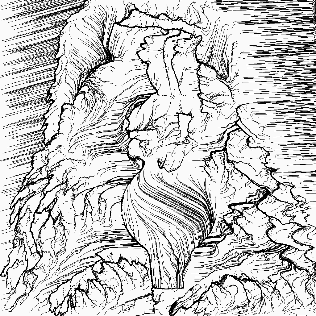
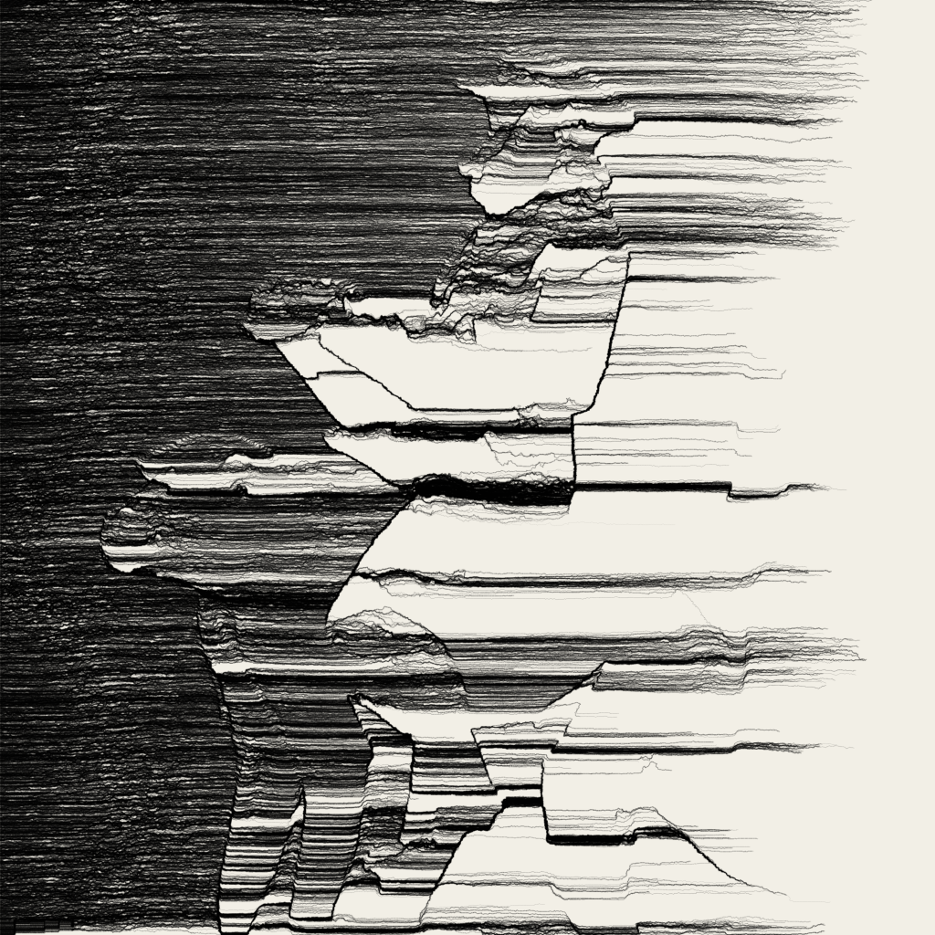
Next, I wanted to explore what happens when I do not use the input image itself but instead its gradient. This means that every pixel was replaced by the absolute difference between its own gray value and that of its neighboring pixels. The result is a high-pass filter, which reveals the edges of an image while hiding the solid-colored areas. Simultaneously, I found that the lines look more like pencil drawings if they have random transparency. You can see both updates in the baboon image below.
Although the high-pass filtered results were interesting, I preferred the chaotic nature of the original input images. The next logical step was to introduce color, which I achieved using the HSB system, a choice that any sensible visual artist should make. This system includes the hue, saturation, and brightness, making it easier to handle than the RGB system. Before plotting the colored lines, I drew slightly thicker black lines and even thicker semi-transparent lines underneath to create softened dark outlines.
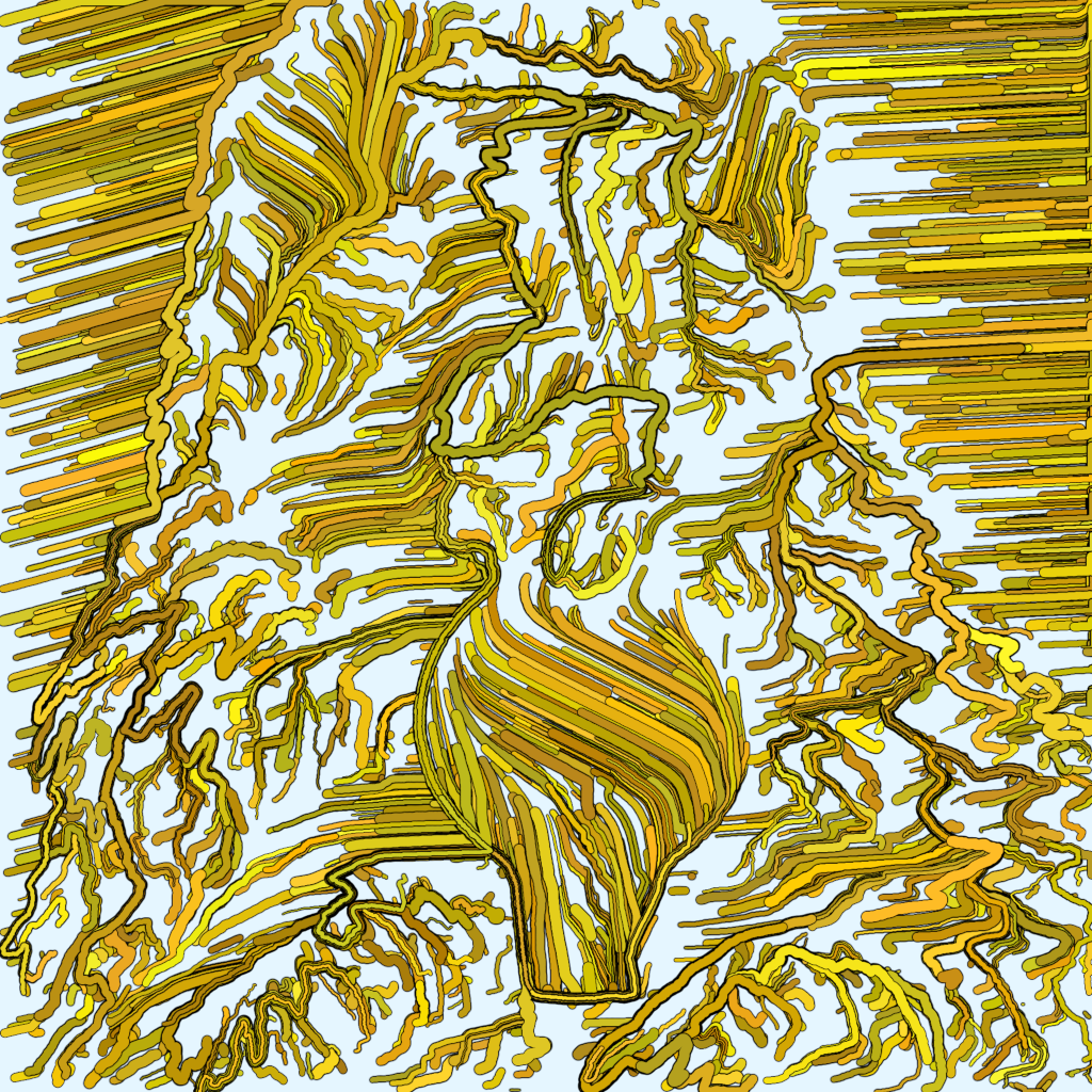
Since a single color can become dull over time, and because I had neglected this aspect for a while, I followed Hobbs’s advice and created some pleasant color palettes, each consisting of about five harmonious colors. To be honest, I’m not yet artistically inclined enough, so I relied on various websites to organize these palettes and selected the ones I liked best.
Additionally, I attempted to reduce the number of overlapping lines by implementing a collision map. This map causes lines to stop if they collide with another line. The difference may be subtle but it significantly reduced computation time.
Becoming bored with my baboon test images and still looking for ways to actively influence the flow fields, I generated new images with Stable Diffusion. Motifs I particularly liked included female models, some of whom were pregnant. Their curves complemented the curves introduced by the gradient-colored backgrounds.
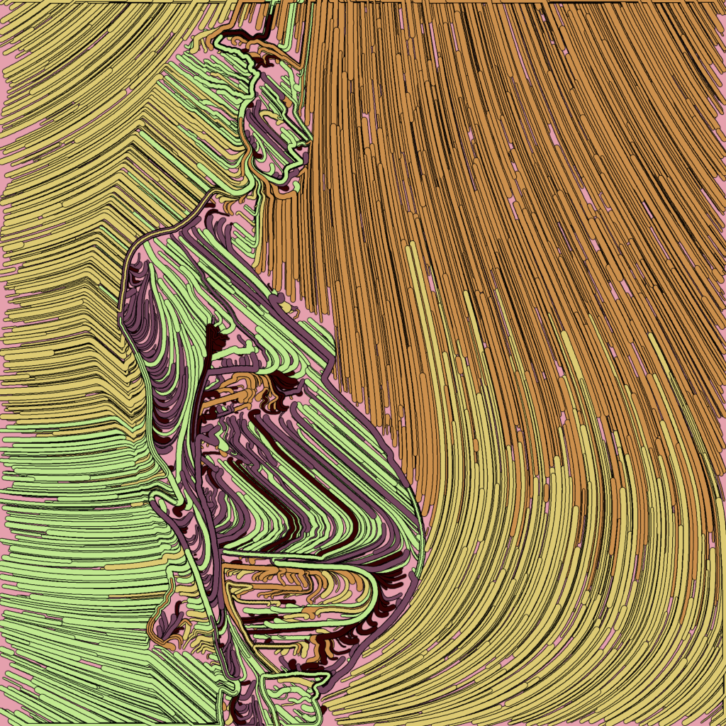
Uniform distribution has the disadvantage that there is no minimum distance between sampled points, which can lead to a lot of overlap and, due to my newly added collision map, the cancellation of too many lines. A tried and tested solution is to use a different starting distribution, such as a Poisson disk sampler as proposed by Robert Bridson and implemented in Processing by Sighack. Without delving into technical details here, this distribution enforces a minimum distance between starting points as well as a maximum distance, which is twice the minimum.
Also, notice how vignette effects on the input image create circular line patterns around the car.
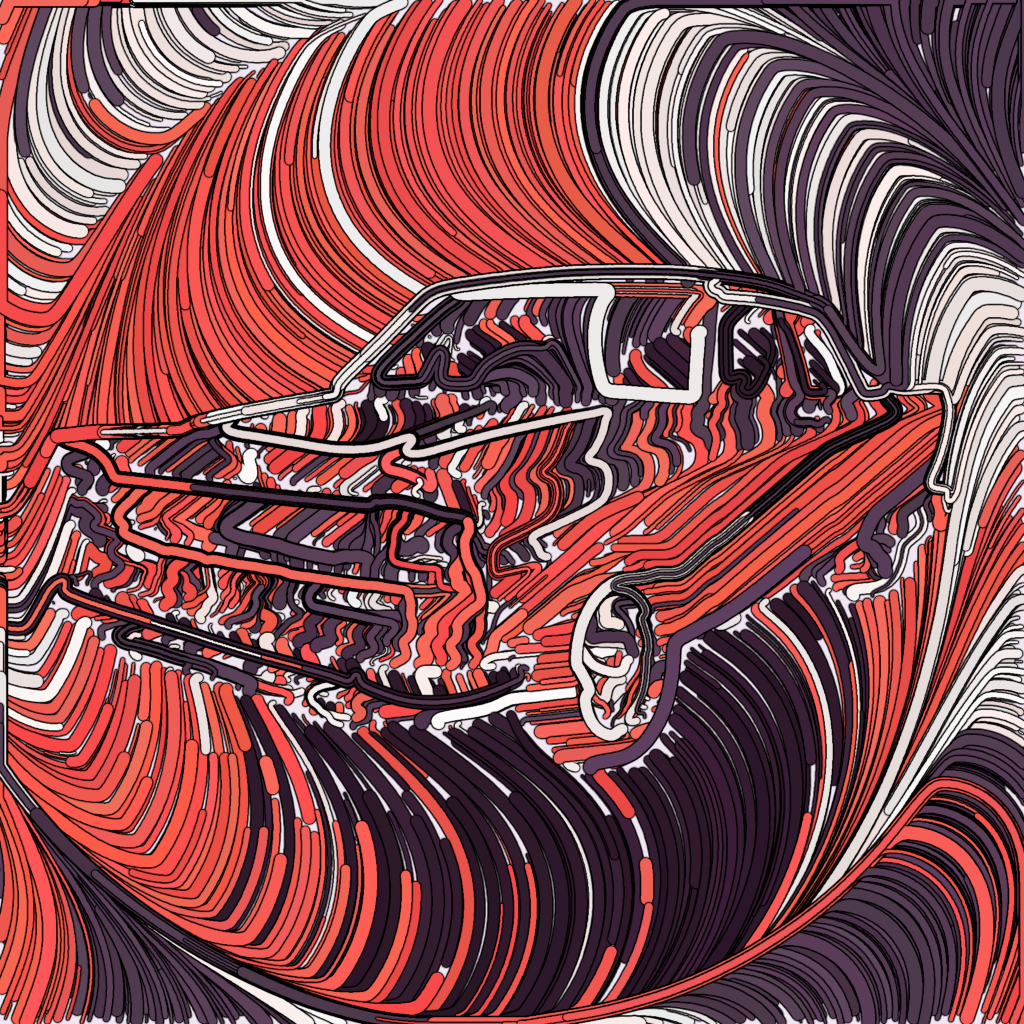
Naturally, ClayGrinder works well with computer graphics due to their uniform faces and clear-cut shapes and edges. In contrast, photos are less suitable due to their heterogeneity and higher levels of noise. I discovered that classic cars against simple backgrounds, reminiscent of advertisements from the 1960s, make ideal input images because they feature both straight and organic lines, and their monochromatic nature typically sets them apart from the background.
Meanwhile, I continuously added new color palettes to my collection and began to dislike some of the ones I added earlier. Eventually, I wrote a Python script that imported the Processing script, including the palettes. This script transformed it into another Python script containing the palettes as a dictionary (along with my own rating system), and would then transform it back into a Processing script containing my favorite palettes. It might sound complicated, but I hope I can reuse it for some other project.
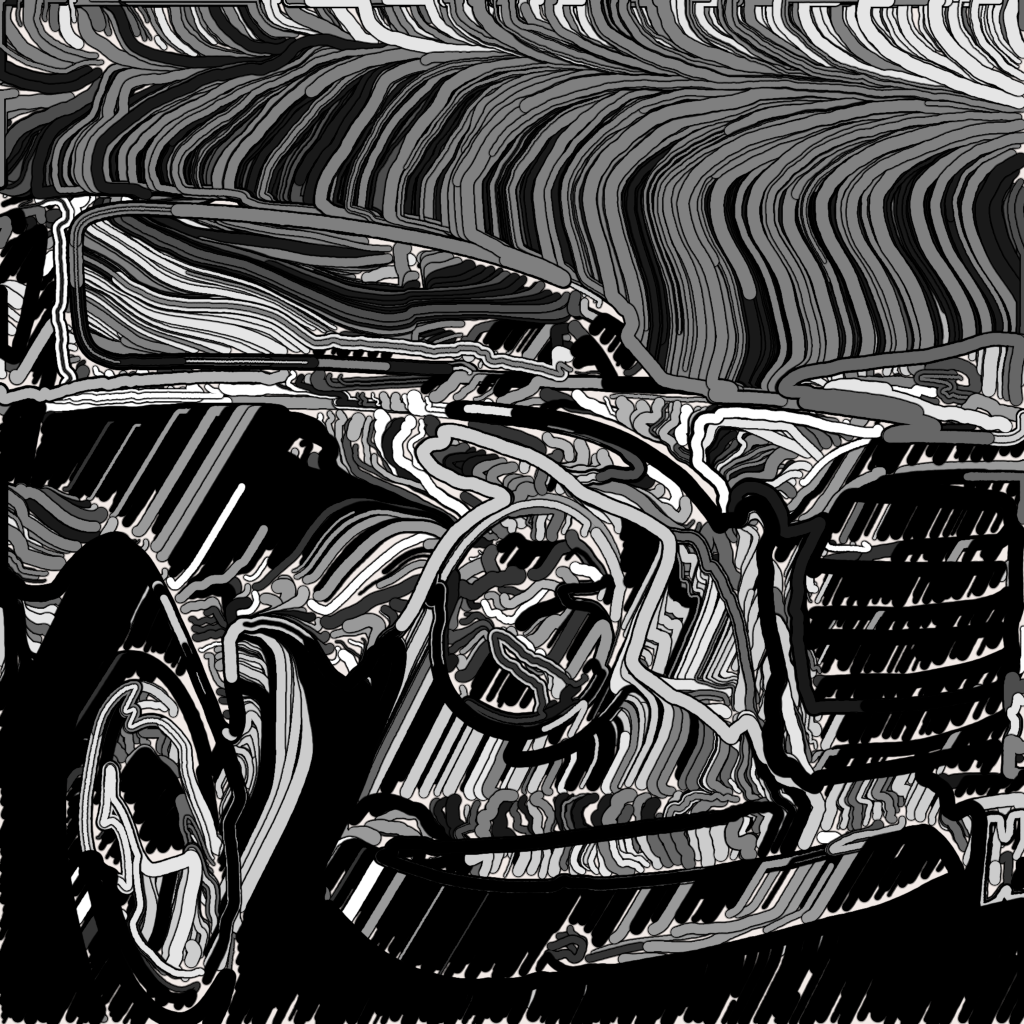
As you can see, I also used grayscale palettes. I am uncertain about the margins, i.e., how the lines behave near the image boundaries. Hobbs prefers to extend his flow fields beyond the visible boundaries; in my case, simply trimming the image margins would suffice.
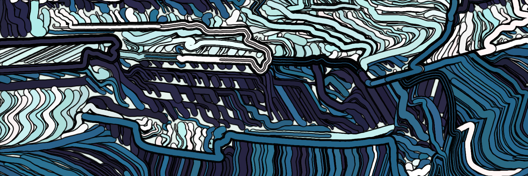
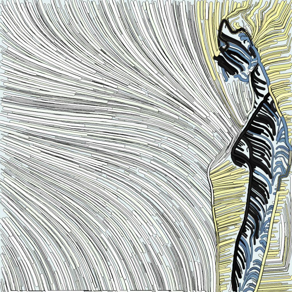
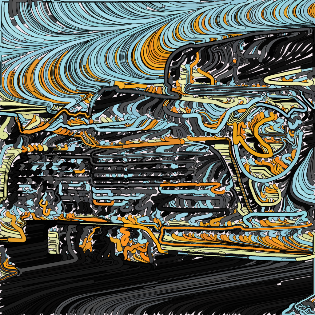
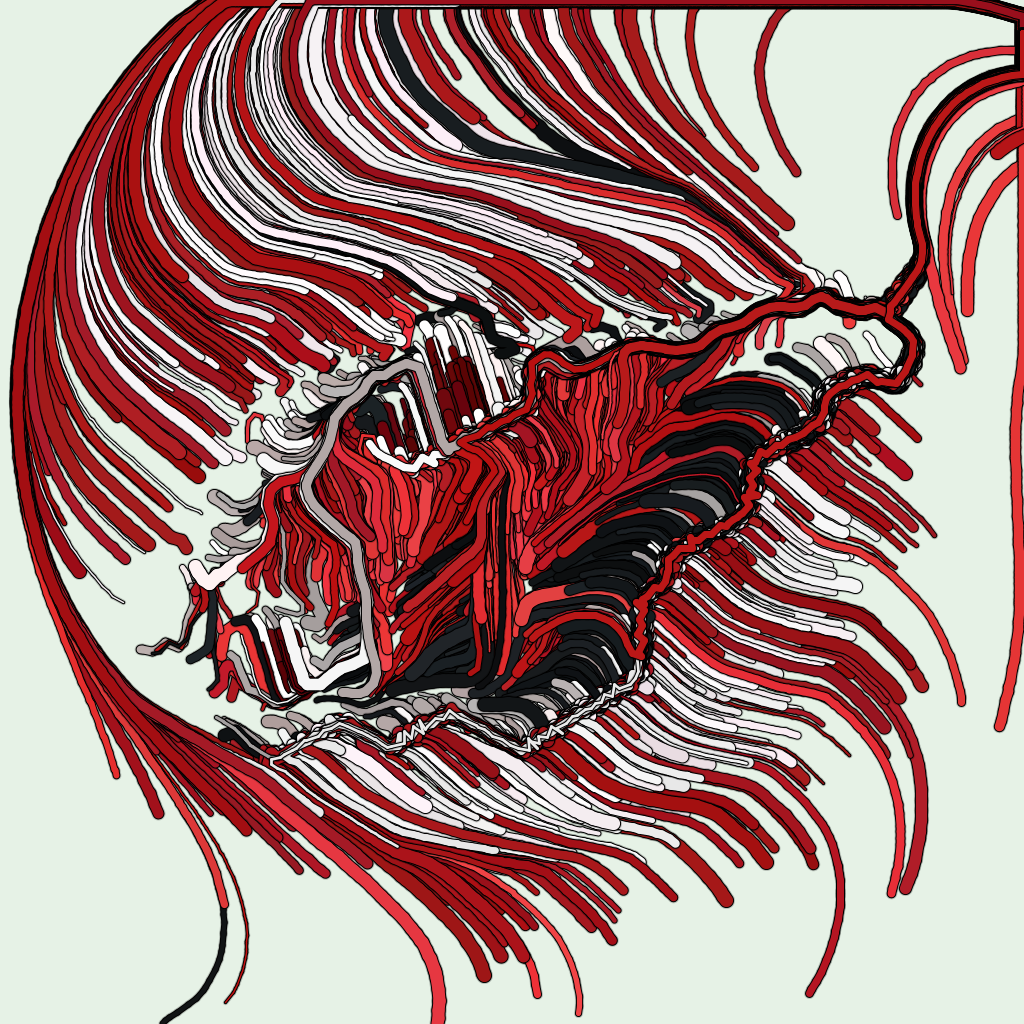
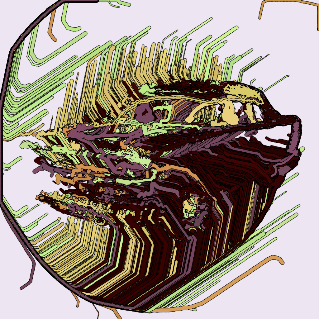
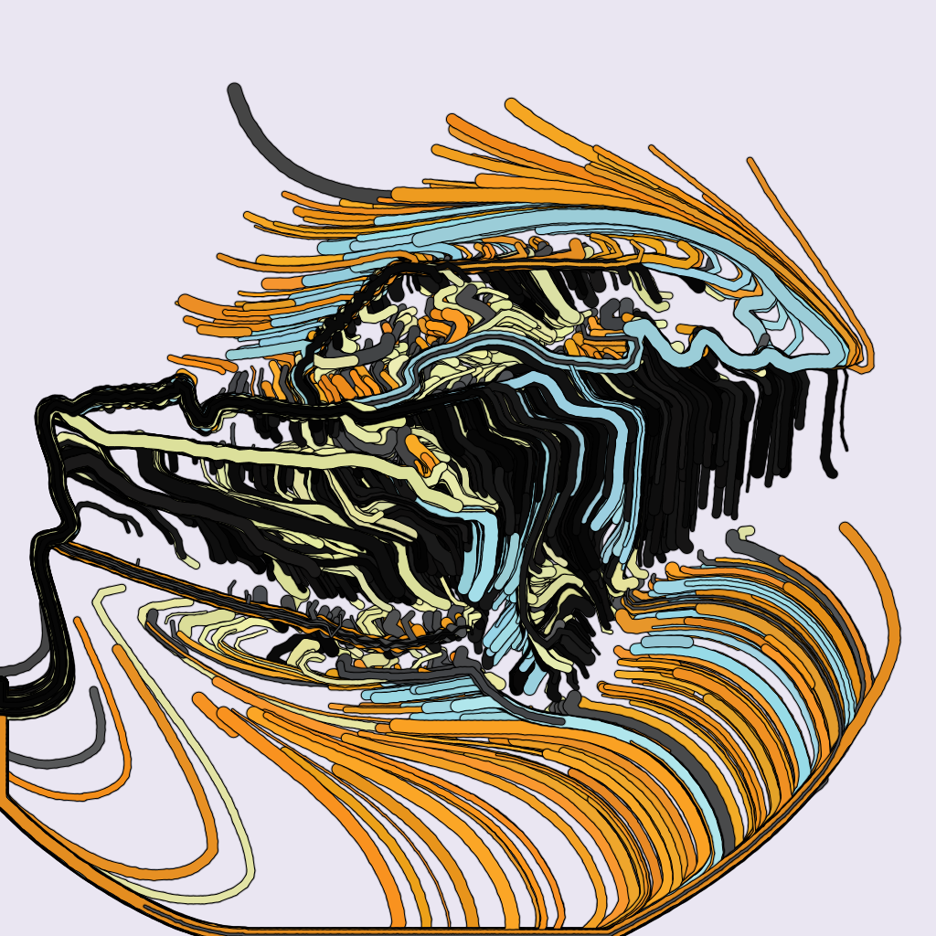
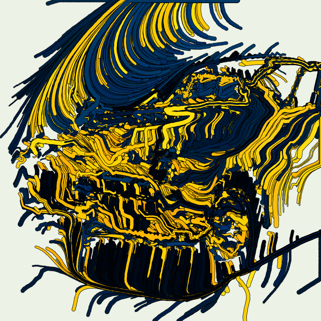
For the final version of ClayGrinder, I used a third starting distribution for the lines, namely the Gaussian distribution. This places many points in the center and fewer points around it, emphasizing the center object by displaying more of the blank background. Furthermore, I experimented with discretized angles, allowing the flow field to assume only a specified number of angles and rounding all values to the nearest valid angle. This results in images that appear even more organized.
One thing I did far too late was to uncouple the image output size from the other size parameters, such as line length or thickness. This led to images looking different when I changed the output resolution, which was crucial for creating high-quality images. Therefore, I changed the entire script to use one unit size, upon which all other parameters depended. With this ultimate update, I was able to create images with 256 megapixels, suitable for posters and art prints.
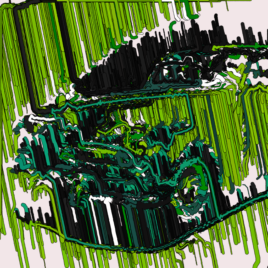
Below, I have shared some of my personal favorites, although the potential range of output images is far greater and nowhere near being exhausted, as it also depends on the input images, of which I surveyed only a small subset.
Leave a Reply