


This is one of the few projects that I spent several years on, and I doubt that I will ever develop something as difficult. The years are 2015 to 2018, and while I had a decent amount of coding experience with Visual Basic and C, this is the one project that taught me how to program. In fact, this project was so important for me that I got a tattoo to always remember it, always reminisce about my time as a master’s student at the Institute for Machine Tools and Factory Management at Technische Universität Berlin. The multi-body brushing simulation was a core element for the dissertation of my academic predecessor Dr.-Ing. Christian Sommerfeld, and I had the honor of cooking it up. There were several times where I threw in the towel, only to come back later and tackle the problem with all my mind could muster in altered and unaltered states: physics, mechanics, analysis, algebra, numerics, visual thinking, programming, planning – even production engineering, the eventual application.
[Source: Machines 2020, 8(4), 89; https://doi.org/10.3390/machines8040089]
In a nutshell, rotating brushing tools do various industrial tasks, such as making surfaces smoother or edges rounder. However, the interactions between the individual bristles (we call them filaments) are extremely complex. Yet it is crucial to fully understand brushing tools in order to improve industrial brushing processes. Tackling the problem with experiments is possible, focusing on single filaments or entire brushing tools, but gives little insight into interaction forces and filament motions. That is where the simulation comes in. The key questions were:
- How are the flexible filaments moving?
- What forces do they exert onto each other and onto the workpiece?
- How are both influenced by the workpiece shape?
As we had to start somewhere, there were several previous models. The first attempt was based on quasi-static elastic beam theory to model single filaments at negligible velocities, as described in my predecessor’s predecessor’s (Dr.-Ing. Leif Hochschild’s) dissertation. We then switched over to Lagrange mechanics and eventually Hertzian contact theory. The tipping point was when I solved the two differential equations for the generalized (and spherical!) coordinates using just pen and paper – before canceling, the equations were eight pages long. I hacked the remaining three pages into MATLAB and for some magic reason got it to work. This was my job as a student worker. For my master’s thesis, I then implemented filament interactions and did some experiments on rotating filaments with a high-speed camera to improve the damping properties.

While the multi-body system was useful for the modeling of some 300 filaments on a flat surface, the computational costs and the fact that it was implemented in slow/interpreted MATLAB posed limitations. That is why I switched to a different modeling method in 2020, using Rocky DEM (today: Ansys Rocky) which is commercially available. Since I did not cook up the math myself, I focused more on how to accurately recognize and model filament patterns for my own dissertation. The state of the art, I dare say, is simulating several rotations of an entire brush tool with tens of thousands of filaments in just a few hours, predicting contact forces and areas with at least 90% accuracy. But this is another topic for another post, so let us stick with the multi-body system. Below are the key features of the simulation.

Filament Discretization
Instead of treating the filament as a continuous flexible rod, the simulation uses a finite segment model. Each filament is discretized into a chain of n rigid cylindrical bodies. The flexibility of the real filament is captured by modeling spring-like joints between these rigid segments.
The state of the entire system is described using generalized coordinates within the framework of Lagrangian Dynamics. For each segment k in the chain, its orientation relative to the previous segment is defined by two angles: a polar angle theta(k) and an azimuthal angle phi(k). The collection of all theta and phi values for all filaments, along with their time derivatives (thetap and phip), defines the complete state of the system at any given moment.
Lagrangian Equations of Motion
The core of the simulation, dgl_lagrange.m, uses Lagrange’s equations of the 2. kind to derive the equations of motion. This is a powerful method that works with scalar energy quantities (i.e., kinetic and potential energy) rather than vector forces. The resulting equation for the system takes the form:
M(q,q’) ⋅ q” = fext − finer − fdamp − fstiff
where:
- q is the vector of all generalized coordinates (all
thetaandphiangles). - q’ is the vector of generalized velocities.
- q” is the vector of generalized accelerations.
- M(q,q’) is the Mass Matrix, calculated by
build_mass.m. This matrix is a function of the system’s current configuration (q), meaning it changes as the filaments bend and deflect. It relates the accelerations to the generalized forces. - The right-hand side represents all generalized forces acting on the system, which are assembled by
build_inhomo.m:- fext: External generalized forces, primarily from gravity.
- fstiff: Internal conservative forces arising from the filament’s own elasticity, modeled as torsional springs with stiffness
Kat each joint. - fshine: Inertial or “fictitious” forces (from the German Scheinkräfte). These are the centrifugal and Coriolis forces that naturally arise because the segments are moving in a rotating, non-inertial reference frame. These terms are velocity-dependent.
- fdamp: Non-conservative dissipative forces, representing the material’s internal damping.

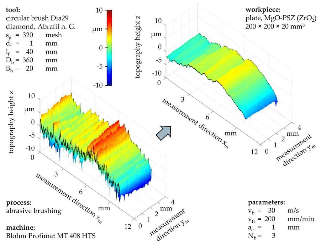
[Source: Ceramics 2021, 4(3), 397-407; https://doi.org/10.3390/ceramics4030029]
Modeling Interactions by Hertzian Contact Theory
- Filament-Workpiece Contact: The interaction with the workpiece, defined by
ws_geometrie.m, is governed byhertz_force.m. When a geometric check (ws_geometrie2.m) detects penetration (d > 0), a repulsive force is generated. You can choose between a simple linear spring model (F∝d) or the more physically accurate Hertzian contact theory, where the force is non-linearly proportional to the penetration depth (F ∝ d1.5 for a spherical tip on a flat plane). This models the local elastic deformation at the contact point. - Inter-Filament Contact:
- Detection (
cylinders_intersect.m): It treats each filament segment as a cylinder and calculates the precise distance between the central axes of any two segments. A collision is detected if this distance indicates a geometric overlap. This is computationally expensive, so aninteraction_matrixis used to pre-determine which filament pairs are close enough to potentially collide, avoiding unnecessary checks. - Force Calculation (
inter_force.m): Once a collision is detected, the resulting force is not just a simple spring. The code provides an extensive library of over 15 established dissipative contact models. While standard Hertz theory is conservative (no energy loss), models like Hunt-Crossley, Lankarani-Nikravesh, or Tsuji et al. add a velocity-dependent term to the force equation. This term represents the energy lost during the collision (due to plasticity, heat, etc.), making the impacts inelastic. The coefficient of restitution (cr_int) is a key parameter here, defining how “bouncy” the collisions are.
- Detection (
In case you are interested in the MATLAB implementation, tell me in the comments and I might upload it on GitHub.
Leave a Reply